In this programming assignment, I implemented my own 2D EKF-SLAM solver in MATLAB. The robot starts with observing the surrounding environment and measuring some landmarks, then executes a control input to move. The measurement and control steps are repeated several times. For simplicity, I assumed the robot observes the same set of landmarks in the same order at each pose. I used EKF-SLAM to recover the trajectory of the robot and the positions of the landmarks from the control input and measurements.

The landmarks are being observed by the robot with a laser sensor which gives bearing angle and range, using which the global coordinates of the landmark are computed. I formulated the measurement Jacobian with respect to the landmark positions and with respect to the robot pose to linearize the set of non-linear equations about the current mean.

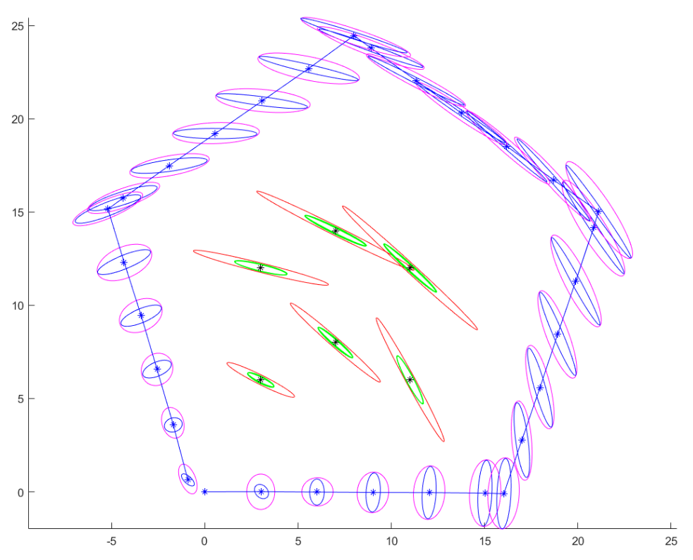
The output figure with each blue “*” representing a position of the robot, and the blue edges showing the estimated trajectory. The uncertainties of the positions of both the robot and the landmarks are shown as 3-sigma error ellipses. In the output figure, the magenta and blue ellipses represent the predicted and updated uncertainties of the robot’s position (orientation not shown here) at each time respectively. Also, the red and green ellipses represent the initial and all the updated uncertainties of the landmarks, respectively.

The EKF-SLAM algorithm estimates the trajectory of the robot and the positions of the landmarks from the control input and measurements. The Kalman gain, computed from the predicted covariance, specifies the degree to which the measurement is incorporated into the new state estimate. If the Kalman Gain is low, the robot trusts that its predicted mean and covariance is reliable, and weights that more heavily while updating the predicted mean and covariance. If the Kalman Gain is high, the robot realises that its predicted uncertainty is higher and weights the latest measurements heavily so as to correct its estimate. Thus, the Kalman gain is a parameter that is used to update the predicted covariance to yield the actual and more accurate covariance of the system. This is why the blue ellipses representing the updated uncertainty of the robot’s position are smaller in area than the magenta ellipses that represent the predicted uncertainty of the robot’s position. The red ellipses that are enclosed by the robot’s trajectory represent the uncertainty in landmark positions at time t = 0. However, as the EKF-SLAM algorithm is executed, the robot is able to update the positions of landmark which are also a part of the state of the system, yielding the smaller green ellipses to model the reduced uncertainty.